Open Method#

강좌: 수치해석

Newton-Raphson Method#

알고리즘#

함수 \(f(x)\) 가 미분 가능하고 연속함수인 경우에 대해서 Taylor Expansion 을 이용하면 다음과 같다.

\[ f(x_{i+1}) = f(x_{i}) + f'(x_i)(x_{i+1} - x_i) + \frac{f''(\xi)}{2!} (x_{i+1} - x_i)^2. \]

여기서 \(\xi \in (x_i, x_{i+1})\) 이다. 선형 근사하고, \(x_{i+1}\) 에서 x 축과 교점이 생기는 경우 다음과 같다.

\[ 0 = f(x_{i+1}) = f(x_{i}) + f'(x_i)(x_{i+1} - x_i). \]

즉, 아래 식을 반복적으로 해석해서 계산할 수 있다.

\[ x_{i+1} = x_{i} - \frac{f(x_i)}{f'(x_i)} \]

종료 판정 기준#

Bracketing method와 동일하게 근사 상대 오차 \(\epsilon_a\) 의 크기가 \(tol\) 보다 작으면 멈춘다.

Note

\(\epsilon_a< tol\) 이면 멈춘다.

예제 1#

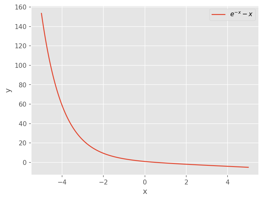
\(f(x) = e^{-x} - x\) 의 근을 구하시오. 초기 가정은 \(x_0 = 0\) 이다.

By Hand#

도함수 \(f'(x) = -e^{-x} - 1\) 이다.

Newton-Raphson 식은 아래와 같다.

\[ x_{i+1} = x_{i} - \frac{f(x_i)}{f'(x_i)} = x_i - \frac{e^{-x} - x}{-e^{-x} - 1} \]

%matplotlib inline
from matplotlib import pyplot as plt

import numpy as np

plt.style.use('ggplot')
plt.rcParams['figure.dpi'] = 150

x = np.linspace(-5, 5, 201)

plt.plot(x, np.exp(-x) - x)
plt.xlabel('x')
plt.ylabel('y')

plt.legend(["$e^{-x} - x$"])

<matplotlib.legend.Legend at 0x7fe95bf43590>

../_images/dbacdcef3b4f6c29ebe526f09af539c2938aff97eab9b3a3922f7c55be420bb6.png

# First Step
x0 = 0
x1 = x0 - (np.exp(-x0) - x0)  / (-np.exp(-x0) - 1)
print("x1 = {:.4f}, err_a = {:.3e}".format(x1, abs((x1 - x0)/x1)))

x1 = 0.5000, err_a = 1.000e+00

# Second step
x0 = x1
x1 = x0 - (np.exp(-x0) - x0)  / (-np.exp(-x0) - 1)
print("x1 = {:.4f}, err_a = {:.3e}".format(x1, abs((x1 - x0)/x1)))

x1 = 0.5663, err_a = 1.171e-01

# Thrid step
x0 = x1
x1 = x0 - (np.exp(-x0) - x0)  / (-np.exp(-x0) - 1)
print("x1 = {:.4f}, err_a = {:.3e}".format(x1, abs((x1 - x0)/x1)))

x1 = 0.5671, err_a = 1.467e-03

# Fourth step
x0 = x1
x1 = x0 - (np.exp(-x0) - x0)  / (-np.exp(-x0) - 1)
print("x1 = {:.4f}, err_a = {:.3e}".format(x1, abs((x1 - x0)/x1)))

x1 = 0.5671, err_a = 2.211e-07

# Bisection Method
from scipy.optimize import root_scalar

f = lambda x: np.exp(-x) - x
root_scalar(f, bracket=[0, 1], method='bisect')

      converged: True
           flag: 'converged'
 function_calls: 41
     iterations: 39
           root: 0.5671432904109679

Quadratic Convergence#

엄밀해를 \(x_r\) 로 가정하자 (\(f(x_r) = 0)\). \(x_i\)를 중심으로 한 Taylor Expansion식을 적용하면 다음과 같다.

\[ 0 = f(x_{r}) = f(x_{i}) + f'(x_i)(x_{r} - x_i) + \frac{f''(\xi)}{2!} (x_{r} - x_i)^2. \]

이 식에서 Newton-Raphson 식을 빼면 다음과 같다.

\[\begin{split} \begin{align} 0 &= f(x_{i}) + f'(x_i)(x_{r} - x_i) + \frac{f''(\xi)}{2!} (x_{r} - x_i)^2 \\ &- f(x_{i}) - f'(x_i)(x_{i+1} - x_i) \\ &= f'(x_i)(x_r - x_{i+1}) + \frac{f''(\xi)}{2!} (x_{r} - x_i)^2 \end{align} \end{split}\]

엄밀해로 부터 오차를 다음과 같이 정의하면

\[ E_i = x_r - x_i, \]

위 식을 아래와 같이 정리할 수 있다.

\[ 0 = f'(x_i) E_{i+1} + \frac{f''(\xi)}{2!} E_i^2 \]

해가 수렴하는 경우 \(x_i, \eta \rightarrow x_r\) 이므로,

\[ E_{i+1} \approx \frac{-f''(x_r)}{2f'(x_r)} E_i^2 = O(E_i^2). \]

즉 현재의 오차는 이전 단계에서의 오차에 제곱에 비례한다.

예제#

위 예제에서 참값은 \(x_r=0.5671432904109679\) 이다. 오차 \(E_i\) 의 변화를 계산해보자.

# Function and derivatives
f = lambda x : np.exp(-x) - x
fp = lambda x: -np.exp(-x) - 1

x0 = x = 0
xr = 0.5671432904109679 

Err = []
itmax = 5
for i in range(itmax):
    # Newton-Raphson
    xn = x - f(x) / fp(x)
    
    # Compute 
    Ei = xr - x
    Err.append(Ei)
    
    x = xn
    print(Ei)

5671432904109679
06714329041096789
0008322872137497273
253761057196101e-07
1868284133242923e-12

-np.exp(-xr) / (2*fp(xr))

0.1809481283173079

위 오차식을 예제에 적용하면

\[ E_{i+1} \approx \frac{-f''(x_r)}{2f'(x_r)} E_i^2 = 0.18095 E_i^2. \]

초기 오차 \(E_0 = x_r - 0\) 이므로, 이 식으로 계산한 오차는 다음과 같다.

매 계산마다 정확한 유효자릿수가 2개가 된다.

# 실제 오차, 추정식
for i in range(1, 5):
    print(Err[i], 0.18095*Err[i-1]**2)

06714329041096789 0.058202841070737574
0008322872137497273 0.0008157626708729342
253761057196101e-07 1.2534442801669386e-07
1868284133242923e-12 2.8443834288658173e-15

예제 2#

아래 함수의 근을 구하시오. 초기값은 0.5로 하자.

\[ f(x) = x^{10} - 1 \]

Newton-Raphson 법을 적용하면 다음과 같다.

\[ x_{i+1} = x_{i} - \frac{f(x_i)}{f'(x_i)} = x_i - \frac{x_i^{10} - 1}{10 x_i^9} \]

# Function and derivatives
f = lambda x : x**10 - 1
fp = lambda x: 10*x**9

x0 = x = 0.5

Err = []
itmax = 45
for i in range(itmax):
    # Newton-Raphson
    xn = x - f(x) / fp(x)
    
    # Compute difference
    Eps = xn - x
    
    x = xn
    print("x1 = {:.4f}, err = {:.3e}".format(x, Eps))

x1 = 51.6500, err = 5.115e+01
x1 = 46.4850, err = -5.165e+00
x1 = 41.8365, err = -4.648e+00
x1 = 37.6529, err = -4.184e+00
x1 = 33.8876, err = -3.765e+00
x1 = 30.4988, err = -3.389e+00
x1 = 27.4489, err = -3.050e+00
x1 = 24.7040, err = -2.745e+00
x1 = 22.2336, err = -2.470e+00
x1 = 20.0103, err = -2.223e+00
x1 = 18.0092, err = -2.001e+00
x1 = 16.2083, err = -1.801e+00
x1 = 14.5875, err = -1.621e+00
x1 = 13.1287, err = -1.459e+00
x1 = 11.8159, err = -1.313e+00
x1 = 10.6343, err = -1.182e+00
x1 = 9.5708, err = -1.063e+00
x1 = 8.6138, err = -9.571e-01
x1 = 7.7524, err = -8.614e-01
x1 = 6.9771, err = -7.752e-01
x1 = 6.2794, err = -6.977e-01
x1 = 5.6515, err = -6.279e-01
x1 = 5.0863, err = -5.651e-01
x1 = 4.5777, err = -5.086e-01
x1 = 4.1199, err = -4.578e-01
x1 = 3.7079, err = -4.120e-01
x1 = 3.3371, err = -3.708e-01
x1 = 3.0034, err = -3.337e-01
x1 = 2.7031, err = -3.003e-01
x1 = 2.4328, err = -2.703e-01
x1 = 2.1896, err = -2.432e-01
x1 = 1.9707, err = -2.189e-01
x1 = 1.7738, err = -1.968e-01
x1 = 1.5970, err = -1.768e-01
x1 = 1.4388, err = -1.582e-01
x1 = 1.2987, err = -1.401e-01
x1 = 1.1784, err = -1.204e-01
x1 = 1.0833, err = -9.500e-02
x1 = 1.0237, err = -5.969e-02
x1 = 1.0023, err = -2.135e-02
x1 = 1.0000, err = -2.292e-03
x1 = 1.0000, err = -2.393e-05
x1 = 1.0000, err = -2.578e-09
x1 = 1.0000, err = 0.000e+00
x1 = 1.0000, err = 0.000e+00

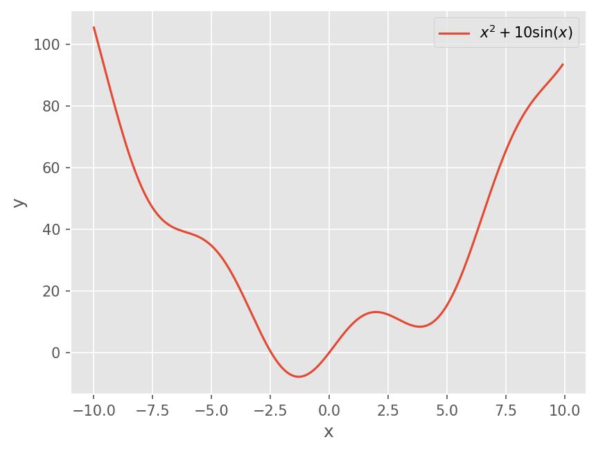
예제 3#

아래 함수의 해를 적절한 초기값으로 부터 근을 구하시오.

\[ f(x) = x^2 + 10 \sin(x) \]

Newton-Raphson 법을 적용하면 다음과 같다.

\[ x_{i+1} = x_{i} - \frac{f(x_i)}{f'(x_i)} = x_i - \frac{x^2 + 10\sin(x)}{2 x + 10\cos(x)} \]

# Function and derivatives
f = lambda x : x**2 + 10*np.sin(x)
fp = lambda x: 2*x + 10*np.cos(x)

x = np.arange(-10, 10, 0.1)

plt.plot(x, f(x))
plt.xlabel('x')
plt.ylabel('y')
plt.legend(["$x^2 + 10\sin(x)$"])

<matplotlib.legend.Legend at 0x7fe95bfb1210>

../_images/5f9c3ba3362cd0d849e82947e601cdcbc021a4e14331a3cfbc72b9edc301b789.png

# 초기값 -4
x0 = x = -4

Err = []
itmax = 5
for i in range(itmax):
    # Newton-Raphson
    xn = x - f(x) / fp(x)
    
    # Compute difference
    Eps = xn - x
    
    x = xn
    print("x1 = {:.4f}, err = {:.3e}".format(x, Eps))

x1 = -2.3787, err = 1.621e+00
x1 = -2.4832, err = -1.045e-01
x1 = -2.4795, err = 3.666e-03
x1 = -2.4795, err = 4.253e-06
x1 = -2.4795, err = 5.736e-12

# 초기값 1
x0 = x = 1

Err = []
itmax = 5
for i in range(itmax):
    # Newton-Raphson
    xn = x - f(x) / fp(x)
    
    # Compute difference
    Eps = xn - x
    
    x = xn
    print("x1 = {:.4f}, err = {:.3e}".format(x, Eps))

x1 = -0.2717, err = -1.272e+00
x1 = 0.0154, err = 2.872e-01
x1 = 0.0000, err = -1.541e-02
x1 = 0.0000, err = -2.251e-05
x1 = 0.0000, err = -5.067e-11

# 초기값 2.5
x0 = x = 2.5

Err = []
itmax = 50
for i in range(itmax):
    # Newton-Raphson
    xn = x - f(x) / fp(x)
    
    # Compute difference
    Eps = xn - x
    
    x = xn
    print("x1 = {:.4f}, err = {:.3e}".format(x, Eps))

x1 = 6.5628, err = 4.063e+00
x1 = 4.5472, err = -2.016e+00
x1 = 3.0957, err = -1.451e+00
x1 = 5.7397, err = 2.644e+00
x1 = 4.3537, err = -1.386e+00
x1 = 2.5082, err = -1.846e+00
x1 = 6.5195, err = 4.011e+00
x1 = 4.5492, err = -1.970e+00
x1 = 3.1005, err = -1.449e+00
x1 = 5.7449, err = 2.644e+00
x1 = 4.3563, err = -1.389e+00
x1 = 2.5186, err = -1.838e+00
x1 = 6.4670, err = 3.948e+00
x1 = 4.5496, err = -1.917e+00
x1 = 3.1014, err = -1.448e+00
x1 = 5.7459, err = 2.645e+00
x1 = 4.3568, err = -1.389e+00
x1 = 2.5206, err = -1.836e+00
x1 = 6.4575, err = 3.937e+00
x1 = 4.5495, err = -1.908e+00
x1 = 3.1010, err = -1.448e+00
x1 = 5.7455, err = 2.644e+00
x1 = 4.3566, err = -1.389e+00
x1 = 2.5197, err = -1.837e+00
x1 = 6.4618, err = 3.942e+00
x1 = 4.5495, err = -1.912e+00
x1 = 3.1012, err = -1.448e+00
x1 = 5.7457, err = 2.645e+00
x1 = 4.3567, err = -1.389e+00
x1 = 2.5201, err = -1.837e+00
x1 = 6.4596, err = 3.939e+00
x1 = 4.5495, err = -1.910e+00
x1 = 3.1011, err = -1.448e+00
x1 = 5.7456, err = 2.645e+00
x1 = 4.3566, err = -1.389e+00
x1 = 2.5199, err = -1.837e+00
x1 = 6.4606, err = 3.941e+00
x1 = 4.5495, err = -1.911e+00
x1 = 3.1011, err = -1.448e+00
x1 = 5.7456, err = 2.645e+00
x1 = 4.3567, err = -1.389e+00
x1 = 2.5200, err = -1.837e+00
x1 = 6.4601, err = 3.940e+00
x1 = 4.5495, err = -1.911e+00
x1 = 3.1011, err = -1.448e+00
x1 = 5.7456, err = 2.645e+00
x1 = 4.3566, err = -1.389e+00
x1 = 2.5200, err = -1.837e+00
x1 = 6.4604, err = 3.940e+00
x1 = 4.5495, err = -1.911e+00

문제점#

수렴하지 않을 수 있다.
- Local extrema 근처에서 진동할 수 있다.
초기 추정 값이 중요함

DIY#

Newton-Raphson method 함수를 구성하시오. 아래 판별 기준을 적용하라.

\(f(x_i)\) 값이 tolerance 보다 작으면 멈춘다.
근사 상대 오차 \(\epsilon_a\) 가 tolerance 보다 작으면 멈춘다.
\(f'(x_i) = 0\) 인 경우 에러를 발생시킨다 (raise ValueError)

def newton(f, fp, x0, rtol=1e-6):
    # DIY
    ...

Secant Method#

Newton-Raphson 방법은 미분 함수 \(f'(x)\) 가 필요하다. 미분을 구하기 힘들 경우 수치적으로 근사한다.

secant-fig — Fig. 10 Secant Method (from Wikipedia)#

그림과 같이 \({i-1}\), \({i}\) 번째 결과로 부터 기울기를 대신 사용한다.

\[ f'(x_i) \approx \frac{f(x_i) - f(x_{i-1})}{x_{i} - x_{i-1}} \]

이 근사 미분값을 사용하는 방법이 Secant method 이다.

\[ x_{i+1} = x_{i} - \frac{f(x_i)}{f'(x_i)} = x_i - \frac{f(x_i)(x_{i} - x_{i-1})}{f(x_i) - f(x_{i-1})} \]

예제 1#

다음 함수 \(f(x) = e^{-x} - x\) 의 근을 구하시오. Secant Method로 해석해보자. (초기 값은 \(x_{-1} = 0, x_0 = 1\) 로 한다.)

# Function and derivatives
f = lambda x : np.exp(-x) - x

xm, x0 = 0.0, 1.0
x = x0

Err = []
itmax = 5
for i in range(itmax):
    # Scecant Method
    xn = x - f(x)*(x - xm) / (f(x) - f(xm))
    
    # Compute difference
    Eps = xn - x
    
    xm = x
    x = xn
    print("x1 = {:.4f}, err = {:.3e}".format(x, Eps))

x1 = 0.6127, err = -3.873e-01
x1 = 0.5638, err = -4.886e-02
x1 = 0.5672, err = 3.332e-03
x1 = 0.5671, err = -2.705e-05
x1 = 0.5671, err = -1.620e-08

예제 2#

다음 함수 \(f(x) = log(x)\) 의 근을 구하시오. Secant Method로 해석해보자. (초기 값은 \(x_{-1} = 0.5, x_0 = 5\) 로 한다.)

# Function and derivatives
f = lambda x : np.log(x)

xm, x0 = 0.5, 5
x = x0

Err = []
itmax = 5
for i in range(itmax):
    # Scecant Method
    xn = x - f(x)*(x - xm) / (f(x) - f(xm))
    
    # Compute difference
    Eps = xn - x
    
    xm = x
    x = xn
    print("x1 = {:.4f}, err = {:.3e}".format(x, Eps))

x1 = 1.8546, err = -3.145e+00
x1 = -0.1044, err = -1.959e+00
x1 = nan, err = nan
x1 = nan, err = nan
x1 = nan, err = nan

/tmp/ipykernel_11119/3825093768.py:2: RuntimeWarning: invalid value encountered in log
  f = lambda x : np.log(x)

root_scalar(f, bracket=[0.5, 5], method='bisect')

      converged: True
           flag: 'converged'
 function_calls: 44
     iterations: 42
           root: 0.9999999999998863

특징#

미분 함수 없이 계산 가능하다.
수렴 속도가 Newton-Raphson과 거의 비슷하나 약간 늦다.
발산할 수 있다.

DIY#

Scecant method 함수를 구성하시오. Newton-Raphson 과 동일한 판별 조건을 사용하자.

def secant(f, x0, x1, rtol=1e-6):
    # DIY
    ...

SciPy 활용#

# root_scalar?

# Function and derivatives
f = lambda x : np.exp(-x) - x
fp = lambda x: -np.exp(-x) - 1

root_scalar(f, fprime=fp, x0=1, method='newton')

      converged: True
           flag: 'converged'
 function_calls: 8
     iterations: 4
           root: 0.5671432904097838

root_scalar(f, x0=0, x1=1, method='secant')

      converged: True
           flag: 'converged'
 function_calls: 7
     iterations: 6
           root: 0.567143290409784

Open Method

Contents

Open Method#

Newton-Raphson Method#

알고리즘#

종료 판정 기준#

예제 1#

By Hand#

Quadratic Convergence#

예제#

예제 2#

예제 3#

문제점#

DIY#

Secant Method#

예제 1#

예제 2#

특징#

DIY#

SciPy 활용#